
Model Interpretability of Deep Neural Networks (DNN) has always been a limiting factor for use cases requiring explanations of the features involved in modelling and such is the case for many industries such as Financial Services. Financial institution whether by regulation or by choice prefer structural models that are easy to interpret by humans that’s why deep learning models within these industries have had slow adoptions. An example of a critical use case would be risk models where usually banks prefer classic statistical methods such as Generalized Linear Models, Bayesian Models and traditional machine learning models such as Tree-based models that are easily explainable and interpret in terms of human intuition.
Interpretability since the beginning has been an important area of research since Deep Learning models can achieve high accuracy but at the expense of high abstraction (i.e. accuracy vs interpretability problem). This is important also because of Trust since a model that is not trusted is a model that will not be used (i.e. try selling to upper management a black box model).
To appreciate this issue just imagine a simple DNN of many layers that is trying to predict an item price using many feature variables and ask yourself:
First, the weights in a neural network are a measure of how strong each connection is between each neuron. So, looking at the first dense layer in your DNN you can tell how strong the connections are between the first layer’s neurons and the inputs. Second, after the first layer you lose the one-to-many relationship and it turns into a monstrous many-to-many entangled mess. This means that a neuron in one layer may be related to some other neuron far away (i.e. neurons experience non-locality effects due to back propagation). Lastly, the weights sure tell the story about the input but the information they have is compressed in the neurons after the application of the activation functions (i.e. non-linearities) making it very difficult to decode. No wonder why Deep Learning models are called black-boxes.
Methods for explaining neural networks generally falls within two broad categories (1) Saliency Methods, and (2) Feature Attribution (FA)
Saliency methods are good at visualizing what is going on inside the network and answering questions such as (1) which weights are being activated given some inputs? or (2) what regions of an image is being detected by a particular convolutional layer? . In our case, this is not what we are after, since it really does not tells us anything about which feature is “best” at describing our final predictions.
FA methods are a type of methods that attempts to fit structural models on a subset of data in such a way as to find out the explanatory power each variable has in the output variable. S. Lundberg, S. Lee, Showed in a NIPS 2017 paper (see paper) that all models Such as LIME, DeepLIFT, and Layer-Wise Relevance Propagation are part of a larger family of methods named Additive Feature Attribution (AFA) methods with the following definition:
Additive Feature Attribution methods have an explanation model that is linear function of binary variables:
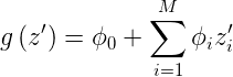
where z’ is a subset of {0,1}^M, where M is the number of simplified features, and Phi_i are weights (i.e. contributions, or the effects).
LIME, DeepLIFT, and Layer-Wise Relevance Propagation all attempts to minimize an objective function to approximate g(z’). So they are all part of the AFA family of methods.
In the same paper, the authors proposed a method for estimating the contributions (Phi_i) of this linear model based on game theory named Shapley values. Why introducing game theory into this picture?
There is a branch of game theory that studies collaborative games in which the goal is to predict the fairest distribution of wealth (i.e. payout) among all players that work together to achieve a common outcome. This happens to be exactly what the authors propose: To use Shapley values as a measure of feature variable contribution towards the prediction of the output of the model.
The authors showed that Shapley values are the optimal solution to a particular type of collaborative games for which AFA methods are also part of (refer to the paper). Lastly, they proposed SHAP (Shapley Additive Explanation) values as a unified measure of feature importance and some methods to efficiently generate them such as:
In this article, I’m going to show you how to use DeepSHAP applied to neural networks but before we start you will have to install the following python library:
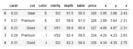
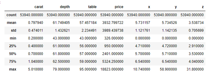
We are going to use the diamonds dataset that comes with seaborn. It is a regression problem for which we are trying to estimate the price of a diamond given diamond quality measures.
Our data looks like:
Let’s get our target and feature variables and encode the categorical variables:
Which gives us the mappings for later use:

Now let’s get our train and test setup:
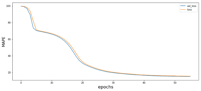
Now let’s set up a neural network model using a simple feed forward fully connected network (with early stopping)
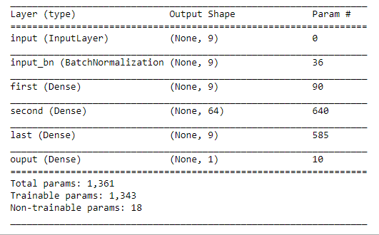
My setup has an NVDIA GPU P4000, so it runs pretty quick, if you don’t have a GPU just increase your batch size based on your memory limitations. So, after 15 sec we get:
Using DeepSHAP is pretty easy thanks to the shap python library. Just set it up as follows :
The method shap_values(X) performs a fitting of the SHAP algorithm based on DeepLIFT using shapley sampling. This takes longer the more data you choose so beware.
Now, let’s see some individual attributions inferred by the model:
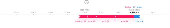
To understand these force plots you need to go back to the author’s paper:
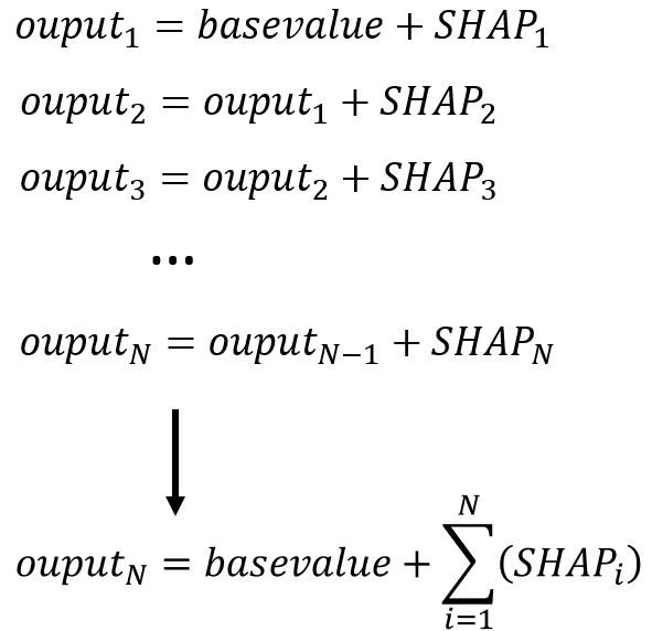
…SHAP (SHapley Additive exPlanation) values attribute to each feature the change in the expected model prediction when conditioning on that feature. They explain how to get from the base value E[f(z)] that would be predicted if we did not know any features to the current output f(x). This diagram shows a single ordering. When the model is non-linear or the input features are not independent, however, the order in which features are added to the expectation matters, and the SHAP values arise from averaging the φi values across all possible orderings.
Notice there is this base value which is the expected value (i.e. E[f(z)]) calculated by DeepSHAP which is just the value that would be predicted if you did not know any features. There is also this output value (i.e. the sumation of all feature contributions and base value) which is equal to the prediction of the actual model. SHAP values, then, just tells you how much contribution each feature adds in order to go from the base value to the output value.
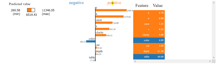
For figure 1, you can understand it as follows:
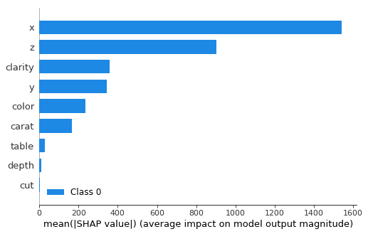
These are all the individual feature contributions to get from the base value to the output value from the record (i.e. individual item in the dataset) displayed as a force plot in figure 1. You can see that there are positive and negative contributions of different magnitude. In this case x,y,z,carat, clarity, cut and depth are all contributing to increase the value from the base value to the value predicted by the model output, whereas color and table contribute to decrease the magnitude from the base value to the prediction. Also, note that the unit of SHAP values is the same as the actual target value (Price).
Here is how you get the output value:
Try adding them and you will see that the output value is equal to the actual model predicted value. This is a very powerful and insightful interpretation method that helps you understand the contributions in terms of target variable units.
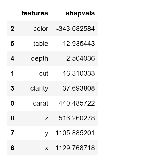
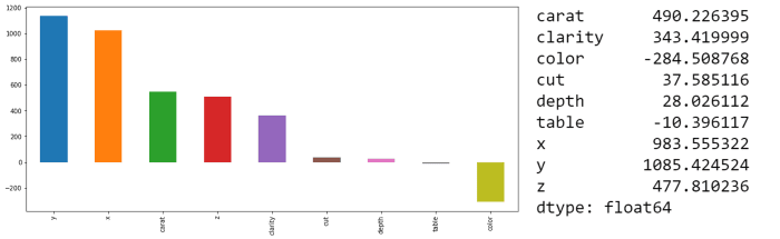
Now, if you want to see the overall contribution of each feature variable you just do:
Plotting the mean values of the contributions gives you Figure 3 which shows you the average contribution of each feature variable to the overall mean model output.
Just for sanity check let’s try an older but also interesting approach.
LIME is an algorithm introduced by a paper “Why Should I Trust You?”: Explaining The Predictions of Any Classifier by Marco Tulio Ribeiro, et al. in 2016.
LIME is a clever algorithm that achieves interpretability of any black box classifier or regressor by performing a local approximation around an individual prediction using an interpretable model (i.e. in this paper case it is a linear model, etc.). That is, it answers the question: Do I trust an individual prediction enough to take an action based on it? So, it is a good algorithm to inspect or debug individual predictions.
SP-LIME is an algorithm that attempts to answer the question Do I trust the model? It does it by framing the problem as a sub-modular optimization problem. That is, it picks a series of instances of the model and their corresponding predictions in a way that is representative of the whole model performance. These picks are performed in such a way that input features that explain more different instances have higher importance score.
We can see that the features x,y,z,carat,clarity, cut, and depth have all positive contributions to the LIME model although in not the same order as SHAP (but they are almost pretty similar). Also, features Table and color have negative contributions to the LIME model confirming as well SHAP values results.
Result from SP-LIME:
To calculate the overall contribution we have to use SP-LIME. It is a little bit more tedious as we have to compute the explanation matrix and get the mean for each feature manually. I use the sample_size of 20 and number of experiments to 5 as the SP optimization algorithm takes a heavy toll in ram.
SP-LIME overall attribution defers a little (although really not that much) from SHAP but keep in mind that I did not optimize the parameters for SP-LIME. It will most likely be in accordance with SHAP if I use a larger sample size and increase the number of experiments run by the SP algorithm as they should since LIME was demonstrated to be an AFA-type algorithm and is an approximation to the Shapley values.
I hope you have learned something new and encourage you to try it in your own datasets with different methods (e.g. DNN, CNN, catboost, etc.). It works also for classification and different types of data such as image data and text data.
